PT_Gtrm

PT_Gtrm: the program for fitting continental conductive geotherms to clouds of PT points according to approximated models of H.N. Pollack & D.S. Chapman (1977) and D. Hasterok D. & D.S. Chapman (2011)

 PT_Gtrm is a freeware program for fitting continental conductive geotherms to clouds of PT points, e.g. to results of geothermobarometric investigations of mantle xenoliths. This program is not intended for simulations of temperature changes with depth: it uses simple but enough precise approximating expressions with physically meaningless coefficients.
 PT_Gtrm approximates two models of continental conductive geotherms:

1. Pollack H.N. & Chapman D.S. On the regional variations of heat flow, geotherms and lithosphere thickness // Tectonophysics, 1977, v.38, n.3-4, p.279-296 DOI:10.1016/0040-1951(77)90215-3
   Chapman D.S. & Pollack H.N. Regional geotherms and lithospheric thickness // Geology, 1977, v.5, n.5, p.265-268 DOI:10.1130/0091-7613(1977)5<265:RGALT>2.0.CO;2
   
2. Hasterok D. & Chapman D.S. Heat production and geotherms for the continental lithosphere // Earth Planet. Sci. Lett., 2011, v.307, n.1-2, p.59–70 DOI:10.1016/j.epsl.2011.04.034
   

 The source data for approximations have been obtained by manual digitizing of diagrams published in original papers. Conversion of depths to pressures has been performed following the simplified model of lithoshere structure with constant density layers:

1. Upper crust (0-16 km), ρ = 2.7 g/cm³
   
2. Middle crust (16-23 km), ρ = 2.85 g/cm³
   
3. Lower crust (23-39 km), ρ = 3.0 g/cm³
   
4. Mantle (>39 km), ρ = 3.3 g/cm³
   

 Densities have been then adjusted for closest correspondence of 40 mW/м² geotherm on the Depth-T diagram in the paper of D. Hasterok and D. Chapman (2011) to the same geotherm on the P–T diagram in the same publication. While these procedures can not be regarded as very precise, approximated geotherms should be enough accurate for their common use on P–T diagrams.

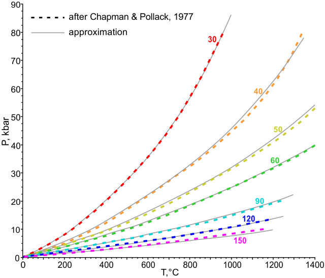
 The family of geotherms by the model of H. Pollack and D. Chapman (1977) down to 40 km (i.e. to the accepted depth of the crust/depleted mantle region transition) is described by the expressions:

P, kbar = a × T°C/(1 - b × T°C)
a = a₀ + a₁ × √mW  + a₂ / mW
b = b₀ + b₁ / mW + b₂ / mW ²

where mW is a heat flow value of interest (in mW/m²), a₀..a₂ and b₀..b₂ are approximation coefficients.

 High-pressure region is expressed as increments to values calculated for the crust/mantle boundary temperatures. These temperatures are defined using the function:

T_max = (t₀ + t₂ × mW) / (1 + t₁ × mW)

 Increments are approximated by the expressions:

ΔP, kbar = c × (T°C - T_max) + d × (T°C - T_max) ³
c = 1 / (c₀ + c₁ × mW + c₂ × mW ³)
d = d₀ + d₁ × mW + d₂ × mW ^2.5 + d₃ × mW ³ + d₄ × e ^-mW

 While these expressions are imprecise for high temperature segments of geotherms near 40–50 mW/m², they should be quite suitable for practical use:




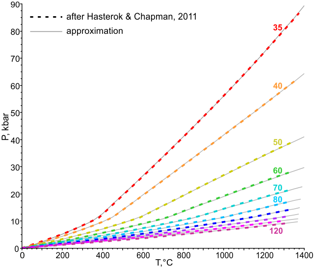
 A similar approximation is used for the family of preferred continental geotherms by the model of D. Hasterok and H. Chapman (2011). Their curves demonstrate sharp bends at the depth of the crust/mantle transition (39 km). Low-pressure segments of geotherms are described by the following expressions:

P, kbar = a × T°C/(1 - b × T°C)
a =a₀ × mW ^a₁
b = b₀ + b₁ × mW ^b₂

 Temperature of the boundary between low- and high-pressure regions can be found by the simple linear equation:

T_max = t₀ + t₁ × mW

 Increments for high-pressure segments are approximated by the expressions:

ΔP, kbar = c × (T°C - T_max) + d × (T°C - T_max) ³
c = 1 / (c₀ + c₁ × mW + c₂ × mW ²)
d = d₀ + d₁ × mW ^d₂

 This approximation fits continental geotherms from Hasterok & Chapman (2011) very well:




 Coefficients for these expressions are stored in the file Special.dat which should be in the directory with the executable PT_Gtrm.exe. This file contains also two coefficients for the linear mantle adiabat expression that can be shown on the diagram, too.

 The program works under operating system of the ©MS Windows family and distributed in the form of ZIP archive. It doesn't have any specially designed installer and is ready for use just after extraction of the archive contents (files PT_GTRM.exe, Special.dat and PT_GTRM.ini) to any desired non-protected directory. NB! If you have working version of the geothermobarometric PTQuick program, it's better to place PT_Gtrm.exe and PT_Gtrm.ini into its directory without overwriting of the existing Special.dat file. A working version of the TriQuick program (designed for diagram graphics) is required for plotting P–T diagrams.

 Press the Paste button in the main program window or double-click in the table area to paste data on P–T points from the clipboard. Data format is a table with TAB-delimited values. If you are working with the ©MS Excel program, just copy desired range of cells to the clipboard and paste it in PT_Gtrm. Tables should have a header (the first line) and two columns (at least) with titles starting from "P," (pressures, in kbar) and "T," (temperatures, °C), with commas. Tables may contain also any other columns, order of columns is not important.

 Notes for PTQuick users: tables generated at calculation of report diagrams are fully compatible with this format and doesn't require any modification before pasting to PT_Gtrm.

 The program performs calculations immediately after the pasting of data and outputs results to the table and on the diagrams:





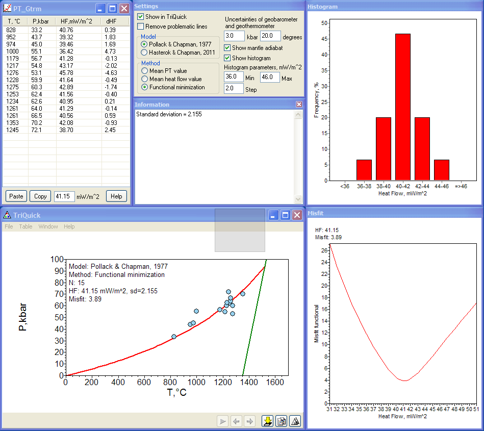
 Geotherm position can be estimated by one of three methods:

1. Mean PT value is the most primitive method: the program calculates heat flow value for the arithmetic mean of pressure and temperature. Its main disadvantage is clearly visible if geotherms are strongly curved while cloud of P–T points forms elongated trend consistent with one of the geotherms. In this case, calculated geotherm will not coincide with expected geotherm and pass at higher pressures.
   

2. Mean heat flow value is also a simple method: the program finds heat flow values for each P–T point, then calculates arithmetic mean. While this method demonstrates smallest standard deviations of heat flow values, calculated geotherms appear shifted to the low pressure side of the cloud of P–T points (i.e. leading to overestimated heat flow value) due to increasing density of geotherms towards low pressures.
   

3. Functional minimization is the most complex method that finds minimum of the following functional proposed in the paper of D. Hasterok and D. Chapman (2011), with two corrected typos(?):
   
   $$Misfit=\sqrt{\frac{1}{N}\sum_{ i=1}^{N}\Big(\frac{\delta P_i^2}{\sigma^2_P}+\frac{\delta T_i^2}{\sigma^2_T}\Big)}$$
   where N is the number of P–T points, δP_i and δT_i are pressure and temperature deviations of the i-th P–T point from the geotherm curve, σ_P and σ_T are uncertainties of geobarometry and geothermometry. The value of Misfit can be defined roughly as a dimensionless equivalent of the average distance between all points and geotherm curve weighted by geothermobarometry uncertainties. It should be noticed that these uncertainties affect mainly absolute functional values and has almost no influence on its minimum position. So, the goal is to find a geotherm demonstrating minimum Misfit value. This method is free of disadvantages mentioned for the two other methods and demonstrates most appropriate results. If this method is selected, the program shows additional diagram with functional values in close vicinity to its minimum. You can copy this diagram to the clipboard: click the diagram by the right mouse button and select Copy in the opened menu.